This article was initially posted at https://discuss.elastic.co/t/dec-23rd-2020-en-new-additions-to-the-keyword-family-constant-keyword-and-wildcard/257213 and https://discuss.elastic.co/t/dec-23rd-2020-es-nuevas-incorporaciones-a-la-familia-de-tipos-keyword-constant-keyword-y-wildcard/257209
We’ve recently introduced two additional keyword types, wildcard and constant_keyword. In this post, we’ll try to introduce them briefly.
The wildcard field is optimized to match any part of string values using wildcards or regular expressions. The usual use case is for security when we might search for a pattern in a process or run grep-like queries on log lines that have not been modeled into different fields.
This was introduced in version 7.9. and we’ll demonstrate this with a basic example. We’ll be using Kibana sample data “Sample weblogs” on a Kibana 7.10.0..
We want to get all the different zip files users downloaded from our website. With the current sample data, we could run the following query:
GET kibana_sample_data_logs/_search?filter_path=aggregations.zip-downloads.buckets.key
{
  "size": 0,
  "_source": "request",
  "query": {
    "wildcard": {
      "url.keyword": {
        "value": "*downloads*.ZIP",
        "case_insensitive": true
      }
    }
  },
  "aggs": {
    "zip-downloads": {
      "terms": {
        "field": "url.keyword",
        "size": 10
      }
    }
  }
}
Which is using the field url.keyword, already existing in the index kibana_sample_data_logs, to run the query. And would return:
{
  "aggregations" : {
    "zip-downloads" : {
      "buckets" : [
        {
          "key" : "https://artifacts.elastic.co/downloads/elasticsearch/elasticsearch-6.3.2.zip"
        },
        {
          "key" : "https://artifacts.elastic.co/downloads/apm-server/apm-server-6.3.2-windows-x86.zip"
        },
        {
          "key" : "https://artifacts.elastic.co/downloads/kibana/kibana-6.3.2-windows-x86_64.zip"
        }
      ]
    }
  }
}
Once we have the index kibana_sample_data_logs, we can update its mappings to add to the existing fields url (type text) and url.keyword (type keyword), a third field url.wirldcard of type wildcard.
PUT kibana_sample_data_logs/_mappings
{
  "properties" : {
        "url" : {
          "type" : "text",
          "fields" : {
            "keyword" : {
              "type" : "keyword",
              "ignore_above" : 256
            },
            "wildcard" : {
              "type" : "wildcard"
            }
          }
        }
      }
}
To populate the field, we can run an update:
POST kibana_sample_data_logs/_update_by_query
Now we can execute the same query using the url.wildcard field.
GET kibana_sample_data_logs/_search?filter_path=aggregations.zip-downloads.buckets.key
{
  "size": 0,
  "_source": "request",
  "query": {
    "wildcard": {
      "url.wildcard": {
        "value": "*downloads*.ZIP",
        "case_insensitive": true
      }
    }
  },
  "aggs": {
    "zip-downloads": {
      "terms": {
        "field": "url.keyword",
        "size": 10
      }
    }
  }
}
What we’ve done is replace a costly leading wildcard query on a keyword field, with a leading wildcard search on a wildcard field.
How does this help us?
- If we have a field with high cardinality, a keyword is not optimized for leading wildcard searches, and thus, it will have to scan all the registries. Wildcard fields index the whole field value using
ngramsand store the entire string. Combining both data structures in the search can speed up the search. - String lengths have a limit. Lucene has a hard limit of 32k on terms, and Elasticsearch imposes an even lower limit. That means the content is dropped from the index if you reach that size. For example, a stack trace can be lengthy. And in some cases, like security, this can create blind spots that are not acceptable.
What you see here is that the same search we had with the keyword field will work on the new wildcard field. In this simple example, the speed will be similar, as we do not have high cardinality in the URL field values for this small data sample. Though you get how it works.
When to use a wildcard? What’s the trade-off? In this post, we won’t get into more details. To further dig into this, go ahead and check the following resources:
- ElasticON Global 2020 talk: Elasticsearch: Introducing the wildcard field
- Blog post: Find Strings within strings faster with the new Elasticsearch wildcard field
Moving on to the second addition to the keyword family, the constant_keyword field, available since version 7.7.0..
This is a field we can use in cases where we want to speed up filter searches.
Usually, the more documents a filter matches, the more that query will cost. For example, if we send all application logs collected for different dev teams to the same index, we might find that later we usually filter them based on the team. If we know this is a usual filter for our use case, we could decide to ingest data on different indices, based on the team field value on each log line. To make queries faster, as they would hit just indices with matching data for that team.
And we can go one step further. Maybe we do not want to change our client’s logic the way they query. We’d like the same queries to work, but still filter out more effectively the indices that have data that won’t match.
If we create those indices with a constant_keyword field, and set the constant in the mappings, the queries sent to all indices will make use of that field to discard indices that won’t match.
We’ll go over it with a basic example to demonstrate how it works.
We’ll create two indices to hold logs for two different teams, A and B. On each index, we define the field team with a constant value, A or B.
PUT my-logs-team-a
{
  "mappings" : {
      "properties" : {
        "@timestamp" : {
          "type" : "date"
        },
        "message" : {
          "type" : "text"
        },
        "team" : {
          "type" : "constant_keyword",
          "value": "A"
        }
      }
    }
}
PUT my-logs-team-b
{
"mappings" : {
"properties" : {
"@timestamp" : {
"type" : "date"
},
"message" : {
"type" : "text"
},
"team" : {
"type" : "constant_keyword",
"value": "B"
}
}
}
}We’ll now ingest a document into each index. We can include the field team value in the document to ingest:
POST my-logs-team-a/_doc/
{
  "@timestamp": "2020-12-04T10:00:13.637Z",
  "message": "239.23.215.100 - - [2018-08-10T13:09:44.504Z] \"GET /apm HTTP/1.1\" 200 8679 \"-\" \"Mozilla/5.0 (X11; Linux i686) AppleWebKit/534.24 (KHTML, like Gecko) Chrome/11.0.696.50 Safari/534.24\"",
  "team": "A"
}
Or leave the value for that field out, letting it take the one defined in the mapping:
POST my-logs-team-b/_doc/
{
  "@timestamp": "2020-12-04T10:01:12.654Z",
  "message": "34.52.49.238 - - [2018-08-10T12:23:20.235Z] \"GET /apm HTTP/1.1\" 200 117 \"-\" \"Mozilla/5.0 (X11; Linux i686) AppleWebKit/534.24 (KHTML, like Gecko) Chrome/11.0.696.50 Safari/534.24\""
}
We will now be able to run the queries in a more efficient way without selecting the indices that contain the values we want to filter. We can search on my-logs-team-*, and Elasticsearch will do its magic for us:
GET my-logs-team-*/_search
{
"query": {
"bool": {
"filter": [
{
"term": {
"team": "B"
}
}
]
}
}
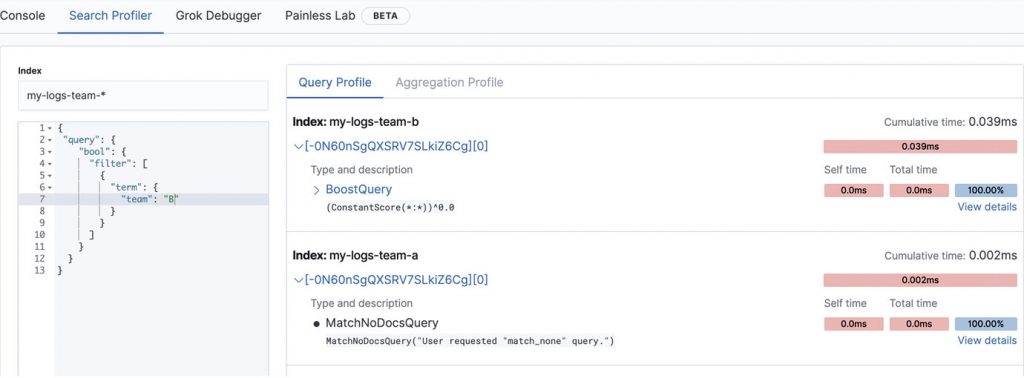
}If we run the query on Kibana’s “Search Profiler”, we can see that when searching for team B, we are executing a match_none query on the team-a index. Thus speeding up the filtering operation.
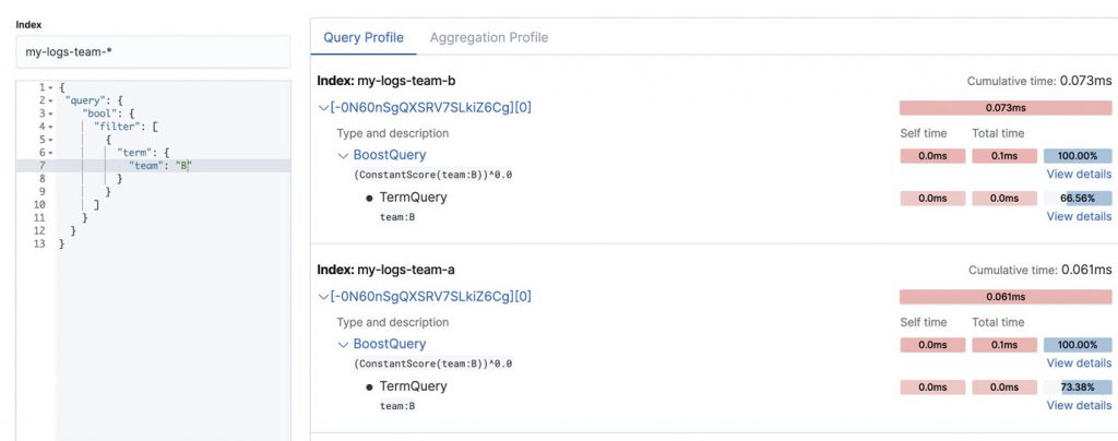
If we created the indices using a type keyword and ran the same test, we would see how both indices run the same term query, even if one of them will return no results.
Go take the two new keyword types for a spin, and let us know how it goes!